Systems linear equations, for which all free terms are equal to zero are called homogeneous :
Any homogeneous system is always consistent, since it always has zero (trivial ) solution. The question arises under what conditions will a homogeneous system have a nontrivial solution.
Theorem 5.2.A homogeneous system has a nontrivial solution if and only if the rank of the underlying matrix is less than the number of its unknowns.
Consequence. A square homogeneous system has a nontrivial solution if and only if the determinant of the main matrix of the system is not equal to zero.
Example 5.6. Determine the values of the parameter l at which the system has nontrivial solutions, and find these solutions:
Solution. This system will have a non-trivial solution when the determinant of the main matrix is equal to zero:
Thus, the system is non-trivial when l=3 or l=2. For l=3, the rank of the main matrix of the system is 1. Then, leaving only one equation and assuming that y=a And z=b, we get x=b-a, i.e.
For l=2, the rank of the main matrix of the system is 2. Then, choosing the minor as the basis:
we get a simplified system
From here we find that x=z/4, y=z/2. Believing z=4a, we get
The set of all solutions of a homogeneous system has a very important linear property : if columns X 1 and X 2 - solutions to a homogeneous system AX = 0, then any linear combination of them a X 1 + b X 2 will also be a solution to this system. Indeed, since AX 1 = 0 And AX 2 = 0 , That A(a X 1 + b X 2) = a AX 1 + b AX 2 = a · 0 + b · 0 = 0. It is because of this property that if a linear system has more than one solution, then there will be an infinite number of these solutions.
Linearly independent columns E 1 , E 2 , E k, which are solutions of a homogeneous system, are called fundamental system of solutions homogeneous system of linear equations if the general solution of this system can be written as a linear combination of these columns:
If a homogeneous system has n variables, and the rank of the main matrix of the system is equal to r, That k = n-r.
Example 5.7. Find the fundamental system of solutions to the following system of linear equations:
Solution. Let's find the rank of the main matrix of the system:
Thus, the set of solutions to this system of equations forms a linear subspace of dimension n-r= 5 - 2 = 3. Let’s choose minor as the base
Then, leaving only the basic equations (the rest will be a linear combination of these equations) and the basic variables (we move the rest, the so-called free variables to the right), we obtain a simplified system of equations:
Believing x 3 = a, x 4 = b, x 5 = c, we find
Believing a= 1, b = c= 0, we obtain the first basic solution; believing b= 1, a = c= 0, we obtain the second basic solution; believing c= 1, a = b= 0, we obtain the third basic solution. As a result, the normal fundamental system of solutions will take the form
Using the fundamental system, the general solution of a homogeneous system can be written as
X = aE 1 + bE 2 + cE 3. a
Let us note some properties of solutions to an inhomogeneous system of linear equations AX=B and their relationship with the corresponding homogeneous system of equations AX = 0.
General solution of an inhomogeneous systemis equal to the sum of the general solution of the corresponding homogeneous system AX = 0 and an arbitrary particular solution of the inhomogeneous system. Indeed, let Y 0 is an arbitrary particular solution of an inhomogeneous system, i.e. AY 0 = B, And Y- general solution of a heterogeneous system, i.e. AY=B. Subtracting one equality from the other, we get
A(Y-Y 0) = 0, i.e. Y-Y 0 is the general solution of the corresponding homogeneous system AX=0. Hence, Y-Y 0 = X, or Y=Y 0 + X. Q.E.D.
Let the inhomogeneous system have the form AX = B 1 + B 2 . Then the general solution of such a system can be written as X = X 1 + X 2 , where AX 1 = B 1 and AX 2 = B 2. This property expresses a universal property of any linear systems in general (algebraic, differential, functional, etc.). In physics this property is called superposition principle, in electrical and radio engineering - principle of superposition. For example, in the theory of linear electrical circuits, the current in any circuit can be obtained as the algebraic sum of the currents caused by each energy source separately.
The linear equation is called homogeneous, if its free term is equal to zero, and inhomogeneous otherwise. System consisting of homogeneous equations, is called homogeneous and has the general form:
It is obvious that every homogeneous system is consistent and has a zero (trivial) solution. Therefore, when applied to homogeneous systems of linear equations, one often has to look for an answer to the question of the existence of nonzero solutions. The answer to this question can be formulated as the following theorem.
Theorem . A homogeneous system of linear equations has a nonzero solution if and only if its rank is less than the number of unknowns .
Proof: Let us assume that a system whose rank is equal has a non-zero solution. Obviously it does not exceed . In case the system has a unique solution. Since a system of homogeneous linear equations always has a zero solution, then the zero solution will be this unique solution. Thus, non-zero solutions are possible only for .
Corollary 1 : A homogeneous system of equations, in which the number of equations is less than the number of unknowns, always has a non-zero solution.
Proof: If a system of equations has , then the rank of the system does not exceed the number of equations, i.e. . Thus, the condition is satisfied and, therefore, the system has a non-zero solution.
Corollary 2 : A homogeneous system of equations with unknowns has a nonzero solution if and only if its determinant is zero.
Proof: Let us assume that a system of linear homogeneous equations, the matrix of which with the determinant , has a non-zero solution. Then, according to the proven theorem, and this means that the matrix is singular, i.e. .
Kronecker-Capelli theorem: An SLU is consistent if and only if the rank of the system matrix is equal to the rank of the extended matrix of this system. A system ur is called consistent if it has at least one solution.Homogeneous system of linear algebraic equations.
A system of m linear equations with n variables is called a system of linear homogeneous equations if all free terms are equal to 0. A system of linear homogeneous equations is always consistent, because it always has at least a zero solution. A system of linear homogeneous equations has a non-zero solution if and only if the rank of its matrix of coefficients for variables is less than the number of variables, i.e. for rank A (n. Any linear combination
Lin system solutions. homogeneous. ur-ii is also a solution to this system.
A system of linear independent solutions e1, e2,...,еk is called fundamental if each solution of the system is a linear combination of solutions. Theorem: if the rank r of the matrix of coefficients for the variables of a system of linear homogeneous equations is less than the number of variables n, then every fundamental system of solutions to the system consists of n-r solutions. Therefore, the general solution of the linear system. one-day ur-th has the form: c1e1+c2e2+...+skek, where e1, e2,..., ek – any fundamental system of solutions, c1, c2,..., ck – arbitrary numbers and k=n-r. The general solution of a system of m linear equations with n variables is equal to the sum
of the general solution of the system corresponding to it is homogeneous. linear equations and an arbitrary particular solution of this system.
7. Linear spaces. Subspaces. Basis, dimension. Linear shell. Linear space is called n-dimensional, if there is a system of linearly independent vectors in it, and any system of a larger number of vectors is linearly dependent. The number is called dimension (number of dimensions) linear space and is denoted by . In other words, the dimension of a space is the maximum number of linearly independent vectors of this space. If such a number exists, then the space is called finite-dimensional. If for anyone natural number n in space there is a system consisting of linearly independent vectors, then such a space is called infinite-dimensional (written: ). In what follows, unless otherwise stated, finite-dimensional spaces will be considered.
The basis of an n-dimensional linear space is an ordered collection of linearly independent vectors ( basis vectors).
Theorem 8.1 on the expansion of a vector in terms of a basis. If is the basis of an n-dimensional linear space, then any vector can be represented as a linear combination of basis vectors:
V=v1*e1+v2*e2+…+vn+en
and, moreover, in the only way, i.e. the coefficients are determined uniquely. In other words, any vector of space can be expanded into a basis and, moreover, in a unique way.
Indeed, the dimension of space is equal to . The system of vectors is linearly independent (this is a basis). After adding any vector to the basis, we obtain a linearly dependent system (since this system consists of vectors of n-dimensional space). Using the property of 7 linearly dependent and linearly independent vectors, we obtain the conclusion of the theorem.
A homogeneous system is always consistent and has a trivial solution  . For a nontrivial solution to exist, it is necessary that the rank of the matrix
  was less than the number of unknowns:
 .
.
Fundamental system of solutions
homogeneous system  call a system of solutions in the form of column vectors
  , which correspond to the canonical basis, i.e. basis in which arbitrary constants
  are alternately set equal to one, while the rest are set to zero.
Then the general solution of the homogeneous system has the form:
Where  - arbitrary constants. In other words, the overall solution is a linear combination of the fundamental system of solutions.
Thus, basic solutions can be obtained from the general solution if the free unknowns are given the value of one in turn, setting all others equal to zero.
Example. Let's find a solution to the system

Let's accept , then we get a solution in the form:

Let us now construct a fundamental system of solutions:
 .
.
The general solution will be written as:

Solutions of a system of homogeneous linear equations have the following properties:

In other words, any linear combination of solutions to a homogeneous system is again a solution.
Solving systems of linear equations using the Gauss method
Solving systems of linear equations has interested mathematicians for several centuries. The first results were obtained in the 18th century. In 1750, G. Kramer (1704–1752) published his works on the determinants of square matrices and proposed an algorithm for finding the inverse matrix. In 1809, Gauss outlined a new solution method known as the method of elimination.
The Gauss method, or the method of sequential elimination of unknowns, consists in the fact that, using elementary transformations, a system of equations is reduced to an equivalent system of a step (or triangular) form. Such systems make it possible to sequentially find all unknowns in a certain order.
Let us assume that in system (1)  (which is always possible).
 (1)
(1)
Multiplying the first equation one by one by the so-called suitable numbers

and adding the result of multiplication with the corresponding equations of the system, we obtain an equivalent system in which in all equations except the first there will be no unknown X 1
 (2)
(2)
Let us now multiply the second equation of system (2) by suitable numbers, assuming that 
 ,
,

and adding it with the lower ones, we eliminate the variable  from all equations, starting from the third.
Continuing this process, after  step we get:
 (3)
(3)
If at least one of the numbers  is not equal to zero, then the corresponding equality is contradictory and system (1) is inconsistent. Conversely, for any joint number system
  are equal to zero. Number
  is nothing more than the rank of the matrix of system (1).
The transition from system (1) to (3) is called straight ahead Gauss method, and finding the unknowns from (3) – in reverse .
Comment : It is more convenient to carry out transformations not with the equations themselves, but with the extended matrix of the system (1).
Example. Let's find a solution to the system
 .
.
Let's write the extended matrix of the system:
 .
.
Let's add the first one to lines 2,3,4, multiplied by (-2), (-3), (-2) respectively:
 .
.
Let's swap rows 2 and 3, then in the resulting matrix add row 2 to row 4, multiplied by  :
:
 .
.
Add to line 4 line 3 multiplied by  :
:
 .
.
It's obvious that  , therefore, the system is consistent. From the resulting system of equations

we find the solution by reverse substitution:
 ,
,
 ,
, ,
, .
.
Example 2. Find a solution to the system:
 .
.

It is obvious that the system is inconsistent, because  , A
, A  .
.
Advantages of the Gauss method :
Less labor intensive than Cramer's method.
Unambiguously establishes the compatibility of the system and allows you to find a solution.
Makes it possible to determine the rank of any matrices.
Kaluga branch of the federal state budgetary educational institution of higher professional education
"Moscow State Technical University named after N.E. Bauman"
(Kharkov Branch of Moscow State Technical University named after N.E. Bauman)
Vlaykov N.D.
Solution of homogeneous SLAEs
Guidelines for conducting exercises
on the course of analytical geometry
Kaluga 2011
Lesson objectives page 4
Lesson plan page 4
Necessary theoretical information p.5
Practical part p.10
Monitoring the mastery of the material covered p. 13
Homework p.14
Number of hours: 2
Lesson objectives:
Systematize the acquired theoretical knowledge about the types of SLAEs and methods for solving them.
Gain skills in solving homogeneous SLAEs.
Lesson plan:
Briefly outline the theoretical material.
Solve a homogeneous SLAE.
Find the fundamental system of solutions of a homogeneous SLAE.
Find a particular solution of a homogeneous SLAE.
Formulate an algorithm for solving a homogeneous SLAE.
Check your current homework.
Carry out verification work.
Present the topic of the next seminar.
Submit current homework.
Necessary theoretical information.
Matrix rank.
Def. The rank of a matrix is the number that is equal to the maximum order among its non-zero minors. The rank of the matrix is denoted by .
If a square matrix is non-singular, then its rank is equal to its order. If a square matrix is singular, then its rank is less than its order.
The rank of a diagonal matrix is equal to the number of its non-zero diagonal elements.
Theor. When a matrix is transposed, its rank does not change, i.e.  .
.
Theor. The rank of a matrix does not change with elementary transformations of its rows and columns.
The theorem on the basis minor.
Def. Minor  matrices
  is called basic if two conditions are met:
a) it is not equal to zero;
b) its order is equal to the rank of the matrix  .
.
Matrix  may have several basis minors.
Matrix rows and columns  , in which the selected basic minor is located, are called basic.
Theor. The theorem on the basis minor. Basic rows (columns) of the matrix  , corresponding to any of its basis minors
  , are linearly independent. Any rows (columns) of the matrix
  , not included in
  , are linear combinations of the basis rows (columns).
Theor. For any matrix, its rank is equal to the maximum number of its linearly independent rows (columns).
Calculating the rank of a matrix. Method of elementary transformations.
Using elementary row transformations, any matrix can be reduced to echelon form. The rank of a step matrix is equal to the number of non-zero rows. The basis in it is the minor, located at the intersection of non-zero rows with the columns corresponding to the first non-zero elements from the left in each of the rows.
SLAU. Basic definitions.
Def. System 

 (15.1)
Numbers  are called SLAE coefficients. Numbers
  are called free terms of equations.
The SLAE entry in the form (15.1) is called coordinate.
Def. A SLAE is called homogeneous if  . Otherwise it is called heterogeneous.
Def. A solution to an SLAE is such a set of values of unknowns, upon substitution of which each equation of the system turns into an identity. Any specific solution of an SLAE is also called its particular solution.
Solving SLAE means solving two problems:
Find out whether the SLAE has solutions;
Find all solutions if they exist.
Def. An SLAE is called joint if it has at least one solution. Otherwise, it is called incompatible.
Def. If the SLAE (15.1) has a solution, and a unique one, then it is called definite, and if the solution is not unique, then it is called indefinite.
Def. If in equation (15.1)  ,The SLAE is called square.
SLAU recording forms.
In addition to the coordinate form (15.1), SLAE records are often used in other representations of it.
 (15.2)
The relation is called the vector form of SLAE notation.
If we take the product of matrices as a basis, then SLAE (15.1) can be written as follows:
 (15.3)
or  .
.
The notation of SLAE (15.1) in the form (15.3) is called matrix.
Homogeneous SLAEs.
Homogeneous system  linear algebraic equations with
  unknowns is a system of the form

Homogeneous SLAEs are always consistent, since there is always a zero solution.
Criterion for the existence of a non-zero solution. For a nonzero solution to exist for a homogeneous square SLAE, it is necessary and sufficient that its matrix be singular.
Theor. If the columns  ,
,
 ,
…,
,
…,
 are solutions to a homogeneous SLAE, then any linear combination of them is also a solution to this system.
Consequence. If a homogeneous SLAE has a non-zero solution, then it has an infinite number of solutions.
It is natural to try to find such solutions  ,
,
 ,
…,
,
…,
 systems so that any other solution is represented as a linear combination of them and, moreover, in a unique way.
Def. Any set of  linearly independent columns
  ,
,
 ,
…,
,
…, , which are solutions of a homogeneous SLAE
  , Where
  - the number of unknowns, and
  - the rank of its matrix
  , is called the fundamental system of solutions of this homogeneous SLAE.
When studying and solving homogeneous systems of linear equations, we will fix the basis minor in the matrix of the system. The basis minor will correspond to basis columns and, therefore, basis unknowns. We will call the remaining unknowns free.
Theor. On the structure of the general solution of a homogeneous SLAE. If  ,
,
 ,
…,
,
…, - arbitrary fundamental system of solutions of a homogeneous SLAE
  , then any of its solutions can be represented in the form
Where  ,
…,
,
…, - some are permanent.
That. the general solution of a homogeneous SLAE has the form
Practical part.
Consider possible sets of solutions of the following types of SLAEs and their graphical interpretation.
 ;
;
 ;
;
 .
.
Consider the possibility of solving these systems using Cramer’s formulas and the matrix method.
Explain the essence of the Gauss method.
Solve the following problems.
Example 1. Solve a homogeneous SLAE. Find FSR.
 .
.
Let's write down the matrix of the system and reduce it to stepwise form.
 .
.
 the system will have infinitely many solutions. The FSR will consist of
  columns.
Let's discard the zero lines and write the system again:
 .
.
We will consider the basic minor to be in the upper left corner. That.  - basic unknowns, and
  - free. Let's express
  through free
  :
:
 ;
;
Let's put  .
.
Finally we have:
 - coordinate form of the answer, or
 - matrix form of the answer, or
 - vector form of the answer (vector - columns are FSR columns).
Algorithm for solving a homogeneous SLAE.
Find the FSR and the general solution of the following systems:
№2.225(4.39)
 . Answer:
№2.223(2.37)
 . Answer:
№2.227(2.41)
 . Answer:
Solve a homogeneous SLAE:
 . Answer:
Solve a homogeneous SLAE:
 . Answer:
Presentation of the topic of the next seminar.
Solving systems of linear inhomogeneous equations.
Monitoring the mastery of the material covered.
Test work 3 - 5 minutes. 4 students participate with odd numbers in the journal, starting from No. 10
|
Follow these steps:
|
Follow these steps:
|
|
|
Calculate the determinant:
|
 ;
;
 ;
;


|
Follow these steps:
|
Follow these steps:
|
|
Find the inverse matrix of this one:
|
Calculate the determinant:
|
 not defined


Homework:
1. Solve problems:
№ 2.224, 2.226, 2.228, 2.230, 2.231, 2.232.
2.Work through lectures on the following topics:
Systems of linear algebraic equations (SLAEs). Coordinate, matrix and vector forms of recording. Kronecker-Capelli criterion for compatibility of SLAEs. Heterogeneous SLAEs. A criterion for the existence of a non-zero solution of a homogeneous SLAE. Properties of solutions of a homogeneous SLAE. Fundamental system of solutions of a homogeneous SLAE, the theorem on its existence. Normal fundamental system of solutions. Theorem on the structure of the general solution of a homogeneous SLAE. Theorem on the structure of the general solution of an inhomogeneous SLAE.
Let's consider homogeneous system m linear equations with n variables:
 (15)
(15)
A system of homogeneous linear equations is always consistent, because it always has a zero (trivial) solution (0,0,…,0).
If in system (15) m=n and , then the system has only a zero solution, which follows from Cramer’s theorem and formulas.
Theorem 1. Homogeneous system (15) has a nontrivial solution if and only if the rank of its matrix is less than the number of variables, i.e. . r(A)< n.
Proof. The existence of a nontrivial solution to system (15) is equivalent to a linear dependence of the columns of the system matrix (i.e., there are numbers x 1, x 2,...,x n, not all equal to zero, such that equalities (15) are true).
According to the basis minor theorem, the columns of a matrix are linearly dependent when not all columns of this matrix are basic, i.e. when the order r of the basis minor of the matrix is less than the number n of its columns. Etc.
Consequence. A square homogeneous system has non-trivial solutions when |A|=0.
Theorem 2. If columns x (1), x (2),…, x (s) are solutions to a homogeneous system AX = 0, then any linear combination of them is also a solution to this system.
Proof. Consider any combination of solutions:
Then AX=A()===0. etc.
Corollary 1. If a homogeneous system has a nontrivial solution, then it has infinitely many solutions.
That. it is necessary to find such solutions x (1), x (2) ,..., x (s) of the system Ax = 0, so that any other solution of this system is represented in the form of their linear combination and, moreover, in a unique way.
Definition. The system k=n-r (n is the number of unknowns in the system, r=rg A) of linearly independent solutions x (1), x (2),…, x (k) of the system Ах=0 is called fundamental system of solutions this system.
Theorem 3. Let a homogeneous system Ах=0 with n unknowns and r=rg A be given. Then there is a set of k=n-r solutions x (1), x (2),…, x (k) of this system, forming a fundamental system of solutions.
Proof. Without loss of generality, we can assume that the basis minor of the matrix A is located in the upper left corner. Then, by the basis minor theorem, the remaining rows of matrix A are linear combinations of the basis rows. This means that if the values x 1, x 2,…, x n satisfy the first r equations, i.e. equations corresponding to the rows of the basis minor), then they also satisfy other equations. Consequently, the set of solutions to the system will not change if we discard all equations starting from the (r+1)th one. We get the system:

Let us move the free unknowns x r +1 , x r +2 ,…, x n to the right side, and leave the basic ones x 1 , x 2 ,…, x r on the left:
 (16)
(16)
Because in this case all b i =0, then instead of the formulas
c j =(M j (b i)-c r +1 M j (a i , r +1)-…-c n M j (a in)) j=1,2,…,r ((13), we get:
c j =-(c r +1 M j (a i , r +1)-…-c n M j (a in)) j=1,2,…,r (13)
If we set the free unknowns x r +1 , x r +2 ,…, x n to arbitrary values, then with respect to the basic unknowns we obtain a square SLAE with a non-singular matrix for which there is a unique solution. Thus, any solution of a homogeneous SLAE is uniquely determined by the values of the free unknowns x r +1, x r +2,…, x n. Consider the following k=n-r series of values of free unknowns:
1, =0, ….,=0,
1, =0, ….,=0, (17)
………………………………………………
1, =0, ….,=0,
(The series number is indicated by a superscript in parentheses, and the series of values are written in the form of columns. In each series =1 if i=j and =0 if ij.
The i-th series of values of free unknowns uniquely correspond to the values of ,,...,basic unknowns. The values of the free and basic unknowns together give solutions to system (17).
Let us show that the columns e i =,i=1,2,…,k (18)
form a fundamental system of solutions.
Because These columns, by construction, are solutions to the homogeneous system Ax = 0 and their number is equal to k, then it remains to prove the linear independence of solutions (16). Let there be a linear combination of solutions e 1 , e 2 ,…, e k(x (1) , x (2) ,…, x (k)), equal to the zero column:
1 e 1 + 2 e 2 +…+ k e k ( 1 X (1) + 2 X(2) +…+ k X(k) = 0)
Then the left side of this equality is a column whose components with numbers r+1,r+2,…,n are equal to zero. But the (r+1)th component is equal to 1 1+ 2 0+…+ k 0= 1 . Similarly, the (r+2)th component is equal to 2 ,…, the kth component is equal to k. Therefore 1 = 2 = …= k =0, which means linear independence of solutions e 1 , e 2 ,…, e k ( x (1) , x (2) ,…, x (k)).
The constructed fundamental system of solutions (18) is called normal. By virtue of formula (13), it has the following form:
 (20)
(20)
Corollary 2. Let e 1 , e 2 ,…, e k-normal fundamental system of solutions of a homogeneous system, then the set of all solutions can be described by the formula:
x=c 1 e 1 +s 2 e 2 +…+с k e k (21)
where с 1,с 2,…,с k – take arbitrary values.
Proof. By Theorem 2, column (19) is a solution to the homogeneous system Ax=0. It remains to prove that any solution to this system can be represented in the form (17). Consider the column X=y r +1 e 1 +…+y n e k. This column coincides with the y column in elements with numbers r+1,...,n and is a solution to (16). Therefore the columns X And at coincide, because solutions of system (16) are determined uniquely by the set of values of its free unknowns x r +1 ,…,x n , and the columns at And X these sets are the same. Hence, at=X= y r +1 e 1 +…+y n e k, i.e. solution at is a linear combination of columns e 1 ,…,y n normal FSR. Etc.
The proven statement is true not only for a normal SDF, but also for an arbitrary SDF of a homogeneous SLAE.
X=c 1 X 1 + c 2 X 2 +…+s n - r X n - r - general solution systems of linear homogeneous equations
Where X 1, X 2,…, X n - r – any fundamental system of solutions,
c 1 ,c 2 ,…,c n - r are arbitrary numbers.
Example. (p. 78)
Let us establish a connection between the solutions of the inhomogeneous SLAE  (1) and the corresponding homogeneous SLAE
  (15)
(15)
Theorem 4. The sum of any solution to the inhomogeneous system (1) and the corresponding homogeneous system (15) is a solution to system (1).
Proof. If c 1 ,…,c n is a solution to system (1), and d 1 ,…,d n is a solution to system (15), then substituting the unknown numbers c into any (for example, i-th) equation of system (1) 1 +d 1 ,…,c n +d n , we get:
B i +0=b i h.t.d.
Theorem 5. The difference between two arbitrary solutions of the inhomogeneous system (1) is a solution to the homogeneous system (15).
Proof. If c 1 ,…,c n and c 1 ,…,c n are solutions of system (1), then substituting the unknown numbers c into any (for example, i-th) equation of system (1) 1 -с 1 ,…,c n -с n , we get:
B i -b i =0 p.t.d.
From the proven theorems it follows that the general solution of a system of m linear homogeneous equations with n variables is equal to the sum of the general solution of the corresponding system of homogeneous linear equations (15) and an arbitrary number of a particular solution of this system (15).
X neod. =X total one +X frequent more than once (22)
As a particular solution to an inhomogeneous system, it is natural to take the solution that is obtained if in the formulas c j =(M j (b i)-c r +1 M j (a i, r +1)-…-c n M j (a in)) j=1,2,…,r ((13) set all numbers c r +1 ,…,c n equal to zero, i.e.
X 0 =(,…,,0,0,…,0) (23)
Adding this particular solution to the general solution X=c 1 X 1 + c 2 X 2 +…+s n - r X n - r corresponding homogeneous system, we obtain:
X neod. =X 0 +C 1 X 1 +C 2 X 2 +…+S n - r X n - r (24)
Consider a system of two equations with two variables:
in which at least one of the coefficients a ij 0.
To solve, we eliminate x 2 by multiplying the first equation by a 22, and the second by (-a 12) and adding them: Eliminate x 1 by multiplying the first equation by (-a 21), and the second by a 11 and adding them: ![]() The expression in parentheses is the determinant
The expression in parentheses is the determinant
Having designated ![]() ,
,![]() , then the system will take the form:, i.e., if, then the system has a unique solution:,.
, then the system will take the form:, i.e., if, then the system has a unique solution:,.
If Δ=0, and (or), then the system is inconsistent, because reduced to the form If Δ=Δ 1 =Δ 2 =0, then the system is uncertain, because reduced to form