A method for solving linear inhomogeneous differential equations of higher orders with constant coefficients by the method of variation of the Lagrange constants is considered. The Lagrange method is also applicable to solving any linear inhomogeneous equations if the fundamental system of solutions of the homogeneous equation is known.
ContentSee also:
Lagrange method (variation of constants)
Consider a linear inhomogeneous differential equation with constant coefficients of an arbitrary nth order:
(1)
.
The method of constant variation, which we considered for the first order equation, is also applicable to equations of higher orders.
The solution is carried out in two stages. At the first stage, we discard the right side and solve the homogeneous equation. As a result, we obtain a solution containing n arbitrary constants. In the second step, we vary the constants. That is, we consider that these constants are functions of the independent variable x and find the form of these functions.
Although we are considering equations with constant coefficients here, but the Lagrange method is also applicable to solving any linear inhomogeneous equations. For this, however, the fundamental system of solutions of the homogeneous equation must be known.
Step 1. Solution of the homogeneous equation
As in the case of first-order equations, we first look for the general solution of the homogeneous equation, equating the right inhomogeneous part to zero:
(2)
.
The general solution of such an equation has the form:
(3)
.
Here are arbitrary constants; - n linearly independent solutions of the homogeneous equation (2), which form the fundamental system of solutions of this equation.
Step 2. Variation of Constants - Replacing Constants with Functions
In the second step, we will deal with the variation of the constants. In other words, we will replace the constants with functions of the independent variable x :
.
That is, we are looking for a solution to the original equation (1) in the following form:
(4)
.
If we substitute (4) into (1), we get one differential equation for n functions. In this case, we can connect these functions with additional equations. Then you get n equations, from which you can determine n functions. Additional equations can be written in various ways. But we will do it in such a way that the solution has the simplest form. To do this, when differentiating, you need to equate to zero terms containing derivatives of functions. Let's demonstrate this.
To substitute the proposed solution (4) into the original equation (1), we need to find the derivatives of the first n orders of the function written in the form (4). Differentiate (4) by applying the rules for differentiating the sum and the product:
.
Let's group the members. First, we write out the terms with derivatives of , and then the terms with derivatives of :
.
We impose the first condition on the functions:
(5.1)
.
Then the expression for the first derivative with respect to will have a simpler form:
(6.1)
.
In the same way, we find the second derivative:
.
We impose the second condition on the functions:
(5.2)
.
Then
(6.2)
.
And so on. Under additional conditions, we equate the terms containing the derivatives of the functions to zero.
Thus, if we choose the following additional equations for the functions :
(5.k) ,
then the first derivatives with respect to will have the simplest form:
(6.k) .
Here .
We find the nth derivative:
(6.n)
.
We substitute into the original equation (1):
(1)
;
.
We take into account that all functions satisfy equation (2):
.
Then the sum of the terms containing give zero. As a result, we get:
(7)
.
As a result, we got a system of linear equations for derivatives:
(5.1)
;
(5.2)
;
(5.3)
;
. . . . . . .
(5.n-1) ;
(7′) .
Solving this system, we find expressions for derivatives as functions of x . Integrating, we get:
.
Here, are constants that no longer depend on x. Substituting into (4), we obtain the general solution of the original equation.
Note that we never used the fact that the coefficients a i are constant to determine the values of the derivatives. That's why the Lagrange method is applicable to solve any linear inhomogeneous equations, if the fundamental system of solutions of the homogeneous equation (2) is known.
Examples
Solve equations by the method of variation of constants (Lagrange).
Solution of examples > > >
Solving higher-order equations by the Bernoulli method
Solving Linear Inhomogeneous Higher-Order Differential Equations with Constant Coefficients by Linear Substitution
 .
.
 .
.The method of variation of an arbitrary constant, or the Lagrange method, is another way to solve first-order linear differential equations and the Bernoulli equation.
Linear differential equations of the first order are equations of the form y’+p(x)y=q(x). If the right side is zero: y’+p(x)y=0, then this is a linear homogeneous 1st order equation. Accordingly, the equation with a non-zero right side, y’+p(x)y=q(x), — heterogeneous linear equation of the 1st order.
Arbitrary constant variation method (Lagrange method) consists of the following:
1) We are looking for a general solution to the homogeneous equation y’+p(x)y=0: y=y*.
2) In the general solution, C is considered not a constant, but a function of x: C=C(x). We find the derivative of the general solution (y*)' and substitute the resulting expression for y* and (y*)' into the initial condition. From the resulting equation, we find the function С(x).
3) In the general solution of the homogeneous equation, instead of C, we substitute the found expression C (x).
Consider examples on the method of variation of an arbitrary constant. Let's take the same tasks as in , compare the course of the solution and make sure that the answers received are the same.
1) y'=3x-y/x
Let's rewrite the equation in standard form (in contrast to the Bernoulli method, where we needed the notation only to see that the equation is linear).
y'+y/x=3x (I). Now we are going according to plan.
1) We solve the homogeneous equation y’+y/x=0. This is a separable variable equation. Represent y’=dy/dx, substitute: dy/dx+y/x=0, dy/dx=-y/x. We multiply both parts of the equation by dx and divide by xy≠0: dy/y=-dx/x. We integrate:
2) In the obtained general solution of the homogeneous equation, we will consider С not a constant, but a function of x: С=С(x). From here
The resulting expressions are substituted into condition (I):
We integrate both parts of the equation:
here C is already some new constant.
3) In the general solution of the homogeneous equation y \u003d C / x, where we considered C \u003d C (x), that is, y \u003d C (x) / x, instead of C (x) we substitute the found expression x³ + C: y \u003d (x³ +C)/x or y=x²+C/x. We got the same answer as when solving by the Bernoulli method.
Answer: y=x²+C/x.
2) y'+y=cosx.
Here the equation is already written in standard form, no need to convert.
1) We solve a homogeneous linear equation y’+y=0: dy/dx=-y; dy/y=-dx. We integrate:
To get a more convenient notation, we will take the exponent to the power of C as a new C:
This transformation was performed to make it more convenient to find the derivative.
2) In the obtained general solution of a linear homogeneous equation, we consider С not a constant, but a function of x: С=С(x). Under this condition

The resulting expressions y and y' are substituted into the condition:
Multiply both sides of the equation by
We integrate both parts of the equation using the integration-by-parts formula, we get:
Here C is no longer a function, but an ordinary constant.
3) Into the general solution of the homogeneous equation
we substitute the found function С(x):
We got the same answer as when solving by the Bernoulli method.
The method of variation of an arbitrary constant is also applicable to solving .
y’x+y=-xy².
We bring the equation to the standard form: y’+y/x=-y² (II).
1) We solve the homogeneous equation y’+y/x=0. dy/dx=-y/x. Multiply both sides of the equation by dx and divide by y: dy/y=-dx/x. Now let's integrate:
We substitute the obtained expressions into condition (II):
Simplifying:

We got an equation with separable variables for C and x:


Here C is already an ordinary constant. In the process of integration, instead of C(x), we simply wrote C, so as not to overload the notation. And at the end we returned to C(x) so as not to confuse C(x) with the new C.
3) We substitute the found function С(x) into the general solution of the homogeneous equation y=C(x)/x:

We got the same answer as when solving by the Bernoulli method.

Examples for self-test:
1. Let's rewrite the equation in standard form: y'-2y=x.
1) We solve the homogeneous equation y'-2y=0. y’=dy/dx, hence dy/dx=2y, multiply both sides of the equation by dx, divide by y and integrate:
From here we find y:
We substitute the expressions for y and y’ into the condition (for brevity, we will feed C instead of C (x) and C’ instead of C "(x)):
To find the integral on the right side, we use the integration-by-parts formula:

Now we substitute u, du and v into the formula:
Here C = const.
3) Now we substitute into the solution of the homogeneous
Method of Variation of Arbitrary Constants
Method of variation of arbitrary constants for constructing a solution to a linear inhomogeneous differential equation
a n (t)z (n) (t) + a n − 1 (t)z (n − 1) (t) + ... + a 1 (t)z"(t) + a 0 (t)z(t) = f(t)
consists in changing arbitrary constants c k in the general decision
z(t) = c 1 z 1 (t) + c 2 z 2 (t) + ... + c n z n (t)
corresponding homogeneous equation
a n (t)z (n) (t) + a n − 1 (t)z (n − 1) (t) + ... + a 1 (t)z"(t) + a 0 (t)z(t) = 0
to helper functions c k (t) , whose derivatives satisfy the linear algebraic system
The determinant of system (1) is the Wronskian of functions z 1 ,z 2 ,...,z n , which ensures its unique solvability with respect to .
If are antiderivatives for taken at fixed values of the constants of integration, then the function
is a solution to the original linear inhomogeneous differential equation. Integration of an inhomogeneous equation in the presence of a general solution of the corresponding homogeneous equation is thus reduced to quadratures.
Method of variation of arbitrary constants for constructing solutions to a system of linear differential equations in vector normal form
consists in constructing a particular solution (1) in the form
where Z(t) is the basis of solutions of the corresponding homogeneous equation, written as a matrix, and the vector function , which replaced the vector of arbitrary constants, is defined by the relation . The desired particular solution (with zero initial values at t = t 0 has the form

For a system with constant coefficients, the last expression is simplified:

Matrix Z(t)Z− 1 (τ) called Cauchy matrix operator L = A(t) .
Consider now the linear inhomogeneous equation
. (2)
Let y 1 ,y 2 ,.., y n be the fundamental system of solutions, and be the general solution of the corresponding homogeneous equation L(y)=0 . Similarly to the case of first-order equations, we will seek a solution to Eq. (2) in the form
. (3)
Let us verify that a solution in this form exists. To do this, we substitute the function into the equation. To substitute this function into the equation, we find its derivatives. The first derivative is  . (4)
. (4)
When calculating the second derivative, four terms appear on the right side of (4), when calculating the third derivative, eight terms appear, and so on. Therefore, for the convenience of further calculations, the first term in (4) is assumed to be equal to zero. With this in mind, the second derivative is equal to  . (5)
. (5)
For the same reasons as before, in (5) we also set the first term equal to zero. Finally, the nth derivative is  . (6)
. (6)
Substituting the obtained values of the derivatives into the original equation, we have  . (7)
. (7)
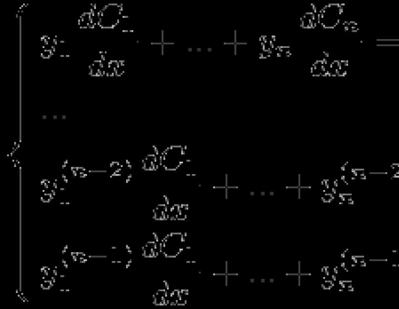
The second term in (7) is equal to zero, since the functions y j , j=1,2,..,n, are solutions of the corresponding homogeneous equation L(y)=0. Combining with the previous one, we obtain a system of algebraic equations for finding the functions C" j (x)  (8)
(8)
The determinant of this system is the Wronsky determinant of the fundamental system of solutions y 1 ,y 2 ,..,y n of the corresponding homogeneous equation L(y)=0 and therefore is not equal to zero. Therefore, there is a unique solution to system (8). Having found it, we obtain the functions C "j (x), j=1,2,…,n, and, consequently, C j (x), j=1,2,…,n Substituting these values into (3), we obtain the solution of the linear inhomogeneous equation.
The described method is called the method of variation of an arbitrary constant or the Lagrange method.
Example #1. Let's find the general solution of the equation y "" + 4y" + 3y \u003d 9e -3 x. Consider the corresponding homogeneous equation y "" + 4y" + 3y \u003d 0. The roots of its characteristic equation r 2 + 4r + 3 \u003d 0 are equal to -1 and - 3. Therefore, the fundamental system of solutions of a homogeneous equation consists of the functions y 1 = e - x and y 2 = e -3 x. We are looking for a solution to an inhomogeneous equation in the form y \u003d C 1 (x)e - x + C 2 (x)e -3 x. To find the derivatives C " 1 , C" 2 we compose a system of equations (8)
C′ 1 ·e -x +C′ 2 ·e -3x =0
-C′ 1 e -x -3C′ 2 e -3x =9e -3x
solving which, we find , Integrating the obtained functions, we have ![]()
Finally we get
Example #2. Solve linear differential equations of the second order with constant coefficients by the method of variation of arbitrary constants: ![]()
y(0) =1 + 3ln3
y'(0) = 10ln3
Solution:
This differential equation belongs to linear differential equations with constant coefficients.
We will seek the solution of the equation in the form y = e rx . To do this, we compose the characteristic equation of a linear homogeneous differential equation with constant coefficients:
r 2 -6 r + 8 = 0
D = (-6) 2 - 4 1 8 = 4
The roots of the characteristic equation: r 1 = 4, r 2 = 2
Therefore, the fundamental system of solutions is the functions: y 1 =e 4x , y 2 =e 2x
The general solution of the homogeneous equation has the form: y =C 1 e 4x +C 2 e 2x
Search for a particular solution by the method of variation of an arbitrary constant.
To find the derivatives of C "i, we compose a system of equations:
C′ 1 e 4x +C′ 2 e 2x =0
C′ 1 (4e 4x) + C′ 2 (2e 2x) = 4/(2+e -2x)
Express C" 1 from the first equation:
C" 1 \u003d -c 2 e -2x
and substitute in the second. As a result, we get:
C" 1 \u003d 2 / (e 2x + 2e 4x)
C" 2 \u003d -2e 2x / (e 2x + 2e 4x)
We integrate the obtained functions C" i:
C 1 = 2ln(e -2x +2) - e -2x + C * 1
C 2 = ln(2e 2x +1) – 2x+ C * 2
Since y \u003d C 1 e 4x + C 2 e 2x, then we write the resulting expressions in the form:
C 1 = (2ln(e -2x +2) - e -2x + C * 1) e 4x = 2 e 4x ln(e -2x +2) - e 2x + C * 1 e 4x
C 2 = (ln(2e 2x +1) – 2x+ C * 2)e 2x = e 2x ln(2e 2x +1) – 2x e 2x + C * 2 e 2x
Thus, the general solution of the differential equation has the form:
y = 2 e 4x ln(e -2x +2) - e 2x + C * 1 e 4x + e 2x ln(2e 2x +1) – 2x e 2x + C * 2 e 2x
or
y = 2 e 4x ln(e -2x +2) - e 2x + e 2x ln(2e 2x +1) – 2x e 2x + C * 1 e 4x + C * 2 e 2x
We find a particular solution under the condition:
y(0) =1 + 3ln3
y'(0) = 10ln3
Substituting x = 0 into the found equation, we get:
y(0) = 2 ln(3) - 1 + ln(3) + C * 1 + C * 2 = 3 ln(3) - 1 + C * 1 + C * 2 = 1 + 3ln3
We find the first derivative of the obtained general solution:
y’ = 2e 2x (2C 1 e 2x + C 2 -2x +4 e 2x ln(e -2x +2)+ ln(2e 2x +1)-2)
Substituting x = 0, we get:
y'(0) = 2(2C 1 + C 2 +4 ln(3)+ ln(3)-2) = 4C 1 + 2C 2 +10 ln(3) -4 = 10ln3
We get a system of two equations:
3 ln(3) - 1 + C * 1 + C * 2 = 1 + 3ln3
4C 1 + 2C 2 +10ln(3) -4 = 10ln3
or
C * 1 + C * 2 = 2
4C1 + 2C2 = 4
or
C * 1 + C * 2 = 2
2C1 + C2 = 2
From: C 1 = 0, C * 2 = 2
A particular solution will be written as:
y = 2e 4x ln(e -2x +2) - e 2x + e 2x ln(2e 2x +1) – 2x e 2x + 2 e 2x


